|
Alfisol, Item 003:
|
LMMpro, version 2.0
The Langmuir Optimization Program
plus
The Michaelis-Menten Optimization Program
|
|

|
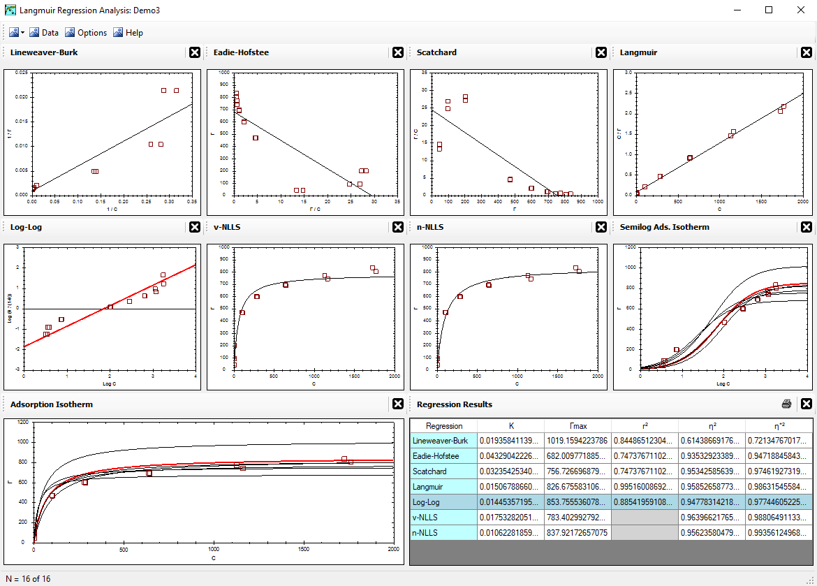
n-NLLS Optimization
The n-NLLS regression method used by LMMpro was presented by Schulthess & Dey in 1996
(Soil Sci. Soc. Am. J. 60:433-442).
n-NLLS stands for normal nonlinear least squares. This regression method optimizes the parameters of the equation
without converting the equation into another form or shape. The best fit is that equation that yields the smallest error.
The error of each datum point is defined as the distance between the datum point and its nearest
point on the parabolic curve. The nearest trajectory of a datum point to the curve is a line that is normal (that is, perpendicular)
to the tangent of the nearest point on the curve.
For the Langmuir Equation, the optimization involves two loops, as follows:
- Make an initial guess of the K and Γmax values.
Let Qi = normal distance of each datum point to the Langmuir isotherm predicted.
The sign of Qi is negative if the point is below or to the right of the curve.
- Let SUM1 = | Σ Qi | = absolute value of the sum of the errors.
- Let SUM2 = Σ Qi2.
- Repeat continuously steps 2 and 3 using a different Γmax value
until a minimum SUM1 value is achieved.
- Repeat continuously steps 2, 3, and 4 using a different K value
until a minimum SUM2 value is achieved.
When you exit both of these loops, you will have the optimized K and Γmax values.
For the Michaelis-Menten Equation, the optimization involves two loops, as follows:
- Make an initial guess of the KM and Vmax values.
Let Qi = normal distance of each datum point to the Michaelis-Menten reaction rate predicted.
The sign of Qi is negative if the point is below or to the right of the curve.
- Let SUM1 = | Σ Qi | = absolute value of the sum of the errors.
- Let SUM2 = Σ Qi2.
- Repeat continuously steps 2 and 3 using a different Vmax value
until a minimum SUM1 value is achieved.
- Repeat continuously steps 2, 3, and 4 using a different KM value
until a minimum SUM2 value is achieved.
When you exit both of these loops, you will have the optimized KM and Vmax values.
Calculating the coordinates of the closest point on the curve.
An exact value of Qi defined above can be calculated as follows.
- Let (m,n) = coordinates of datum point.
Let (r,s) = coordinates of closest point on the predicted curve.
- The distance beween two points is defined by:
|
Q = [ (m - r)2 + (n - s)2 ]0.5
|
- Substitute the theoretical equation for s into the equation above:
|
For Langmuir Equation: |
|
|
For Michaelis-Menten Equation: |
|
- Using differential equations, we solve to minimize Q as a function of r.
That is, dQ/dr = 0. Simplify the result into the following equation of the
fourth degree:
|
A r4 + B r3 + C r2 + D r + E = 0
|
- For the Langmuir Equation:
Let A = K3 .
Let B = 3K2 - mK3 .
Let C = 3K - 3mK2 .
Let D = 1 - 3mK + K2Γmax2 - nK2Γmax .
Let E = - m - nKΓmax .
Note: the definition of D above is correct. It is not correct in the original publication (Schulthess & Dey, 1996).
Also note that n and Γmax are multiplied by the axes conversion factor (ACF) in order to maintain
the parity of the units in each component of this equation of the fourth degree.
- For the Michaelis-Menten Equation:
Let A = KM-3 .
Let B = 3KM-2 - mKM-3 .
Let C = 3/KM - 3mKM-2 .
Let D = 1 - 3m/KM + KM-2Vmax2 -
nKM-2Vmax .
Let E = - m - (n/KM)Vmax .
Note that n and Vmax are multiplied by the axes conversion factor (ACF) in order to maintain
the parity of the units in each component of this equation of the fourth degree.
- Choose the feasible root for the value of r.
The solution to the equation of the fourth degree yields four roots. Only one of these is the feasible answer.
- Once r is known, use Equation [2] and [3] to evaluate the values of s and Q.
Note that the n-NLLS regression will optimize the parameters assuming that minimizing the normal error yields the best results.
This method does not have any known bias in favor of any particular region of the curve. Furthermore, the ACF factor gives
much flexibility to how one wishes to weigh the axes units.
Also note that the n-NLLS regression will result in an optimized curve with the data evenly distributed above and
below the curve. That is, the sum of the errors above the curve will be the same value as the sum of the errors below the curve.
This balance is a result of the SUM1 definition outlined above. While the SUM1 definition balances the data around the curve,
the SUM2 definition tightens the curve to get as close to the data as possible.