|
Alfisol, Item 003:
|
LMMpro, version 2.0
The Langmuir Optimization Program
plus
The Michaelis-Menten Optimization Program
|
|

|
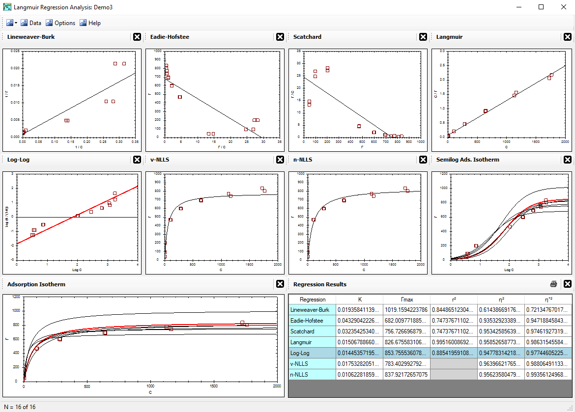
v-NLLS Optimization
The v-NLLS regression method used by LMMpro is based on an adaptation of the optimization method discussed by
Persoff & Thomas in 1988 (Soil Sci. Soc. Am. J. 52:886-889).
v-NLLS stands for vertical nonlinear least squares. This regression method optimizes the parameters of the equation
without converting the equation into another form or shape. The best fit is that equation that yields the smallest error.
The error of each datum point is defined as the vertical difference between the predicted value and the actual value.
The predicted value is the value calculated for a given xi, and the actual value is the value measured
for a given xi.
For the Langmuir Equation, the optimization is as follows:
- Let Σ εi2 =
Σ error2 =
Σ (measured - predicted)2
- Substitute the Langmuir Equation for predicted values:
|
Σ εi2 = Σ [ Γi -
|
Γmax K ci
1 + K ci |
]2
|
|
- Expand the square term:
|
Σ εi2 = Σ [
|
Γmax K ci
1 + K ci |
]2 - Σ [
|
2 Γi Γmax K ci
1 + K ci |
] + Σ Γi2
|
|
- To optimize Γmax, set the first derivative equal to zero and solve:
d(Σ εi2)
dΓmax
|
= 0 = 2 Γmax Σ [
|
K ci
1 + K ci |
]2 - Σ [
|
2 Γi K ci
1 + K ci |
] + 0
|
|
- Solving Equation [4] for Γmax yields:
- If K is known (or fixed by the user), then use Equation [5] above to get the optimized Γmax value.
- If K is not known, guess K values, and then use Equation [5] to get the corresponding best Γmax value.
Finally, use Equation [2] to determine the error that corresponds to the guesses made. Repeat the process by incrementally
increasing or decreasing the K value guesses until the minimum error condition is found.
- If Γmax is known (or fixed by the user), then Equation [5] is not needed. The best value of K, however, is still
determined with Equation [2] and an iteration loop to find the condition with the minimum error.
For the Michaelis-Menten Equation, the optimization is as follows:
- Let Σ εi2 =
Σ error2 =
Σ (measured - predicted)2
- Substitute the Michaelis-Menten Equation for predicted values:
|
Σ εi2 = Σ [ vi -
|
Vmax Si
KM + Si |
]2
|
|
- Expand the square term:
|
Σ εi2 = Σ [
|
Vmax Si
KM + Si |
]2 - Σ [
|
2 vi Vmax Si
KM + Si |
] + Σ vi2
|
|
- To optimize Vmax, set the first derivative equal to zero and solve:
d(Σ εi2)
dVmax
|
= 0 = 2 Vmax Σ [
|
Si
KM + Si |
]2 - Σ [
|
2 vi Si
KM + Si |
] + 0
|
|
- Solving Equation [4] for Vmax yields:
- If KM is known (or fixed by the user), then use Equation [5] above to get the optimized Vmax value.
- If KM is not known,
guess KM values, and then use Equation [5] to get the corresponding best Vmax value.
Finally, use Equation [2] to determine the error that corresponds to the guesses made. Repeat the process by incrementally
increasing or decreasing the KM value guesses until the minimum error condition is found.
- If Vmax is known (or fixed by the user), then Equation [5] is not needed.
The best value of KM, however, is still
determined with Equation [2] and an iteration loop to find the condition with the minimum error.
Note that the v-NLLS regression will optimize the parameters assuming that minimizing the vertical error yields the best results.
This method does have some bias in favor of any region of the curve where the vertical changes are most pronounced.
In other words, for a parabolic equation such as the Langmuir Equation or the
Michaelis-Menten Equation, the v-NLLS regression has some bias toward the lower left region of the graph.
Also note that the v-NLLS regression does not result in an optimized curve with the data evenly distributed above and
below the curve. That is, the sum of the errors above the curve is not the same value as the sum of the errors below the curve.
Least squares regressions will only balance the data around the curve if the function has a constant term.
For example, in y = f(x) + b, b is the constant term. The Langmuir Equation and the Michaelis-Menten Equation are lacking the
contant term (b).